Introduction to Partial Differential Equations - Math 21a Fall 2003

If you took Math 1b here at Harvard, then you have already been introduced to the idea of a differential equation. Up until now, however, if you have already worked with differential equations then they’ve probably all been ordinary differential equations (ODEs), involving “ordinary” derivatives of a function of a single variable. Now that you have worked with functions of several variables in Math 21a, you are ready to explore a new area of differential equations, one that involves partial derivatives. These equations are aptly named partial differential equations (PDEs). During this short section of Math 21a, you will get a chance to see some of the most important PDEs, all of which are examples of linear second-order PDEs (the terminology will be explained shortly).

First, however, in case you haven’t worked with too many differential equations at this point, let’s back up a bit and review some of the issues behind ordinary differential equations.

Ordinary Differential Equations

A differential equation, simply put, is an equation involving one or more derivatives of a function y = f(x). These equations can be as straightforward as

(1) y¢ = 3,

or more complicated, such as

(2) y¢¢ + 12y = 0

(3) (x² y¢¢¢ ) + e^x y¢ – 3xy = (x³ + x).

There are a number of ways of classifying such differential equations. At the least, you should know that the order of a differential equation refers to the highest order of derivative that appears in the equation. Thus these first three differential equations are of order 1, 2 and 3 respectively.

Differential equations show up surprisingly often in a number of fields, including physics, biology, chemistry and economics. Anytime something is known about the rate of change of a function, or about how several variables impact the rate of change of a function, then it is likely that there is a differential equation hidden behind the scenes. Many laws of physics take the form of differential equations, such as the classic force equals mass times acceleration (since acceleration is the second derivative of position with respect to time). Modeling means studying a specific situation to understand the nature of the forces or relationships involved, with the goal of translating the situation into a mathematical relationship. It is quite often the case that such modeling ends up with a differential equation. Clearly one of the main goals of such modeling is to find solutions to such equations, and then to provide some type of understanding or interpretation of the result.

In biology, for instance, if one studies populations (such as of small one-celled organisms), and their rates of growth, then it is easy to run across one of the most basic differential equation models, that of exponential growth. To model the population growth of a group of e-coli cells in a petri dish, for example, if we make the assumption that the cells have unlimited resources, space and food, then it turns out that the cells will reproduce at a fairly specific rate. The trick to figuring out how the cell population is growing is to realize that the number of new cells created over any small time interval is in proportion to the number of cells present at that time.

This means that if we look in the petri dish and see that there are 500 cells at a particular moment, then the number of new cells being created at that time should be 5 times the number of new cells being created if we had looked in the dish and only seen 100 cells (i.e. 5 times the population, 5 times the number of new cells being created). Curiously, this simple observation led to population studies about humans (by Malthus and others in the 19^th century), based on exactly the same idea. Thus, we have a simple observation that the rate of change of the population at any particular time is in direct proportion to the number of cells present at that time. If you now translate this observation into a mathematical statement involving the population function y = P(t), where t stands for time, and P(t) is the function giving the population of cells at time t then you have become a mathematical modeler.

Answer (yielding another example of a differential equation):

(4) P¢ (t) = k P(t), or, equivalently, y¢ = k y

To solve a differential equation means to find a solution function y = f(t), such that when the corresponding derivatives, y¢ , y¢¢, etc. are computed and substituted into the equation, then the equation becomes an identity. For instance, in the first example, equation (1) from above, the differential equation y¢ = 3 is equivalent to the condition that the derivative of the function y = f(x) is a constant, equal to 3. To solve this means to find a function whose derivative with respect to x is constant, and equal to 3. Many such functions come to mind quickly, such as y = 3x, or y = 3x + 5, or y = 3x – 12. Each of these functions is said to satisfy the original differential equation, in that each one is a specific solution to the equation. In fact, clearly anything of the form y = 3x + c, where c is any constant, will be a solution to the equation. And on the other hand, any function that actually satisfies equation (1) will have to be of the form y = 3x + c.

To separate the idea of a specific solution, such as y = 3x + 5, from a more general set or family of solutions, y = 3x + c, with c an arbitrary constant, we call an individual solution function, such as as y = 3x + 5, a specific or particular solution (no surprise there), and call the functions, y = 3x + c, which contain an arbitrary constant (or constants), a general solution.

Note that if someone asked you to solve the differential equation y¢ = 3, then any function of the form y = 3x + c, would do as an answer. However, if the same person asked you to solve y¢ = 3, as well as to find the particular solution that also satisfied another condition, such as y(0) = 20, then the extra condition would force the constant c to be equal to 20. To see this, note that the general solution is y = 3x + c. To find y(0) just substitute in x = 0, so that you find that y(0) = c. Then to make the result equal to 20, according to the extra condition, it must be the case that c equals 20, so that the particular solution to this situation is y = 3x + 20, now with no arbitrary constants remaining.

An extra condition in addition to a differential equation, is called an initial condition, if the condition involves the value of the function when x = 0 (or t = 0, or whatever the independent variable is labeled for the function in the given situation). Sometimes to identify a specific solution to an ODE, several initial conditions need to be given, not just about the value of the function, y = f(x), when x = 0, but also giving the value of derivatives of y when x = 0. This will often happen, for instance, if the differential equation involves derivatives of higher order. In fact, typically the order of the highest derivative that shows up in the equation will equal the number of constants that show up in the general solution to a differential equation (think of solving the equation as involving as many integrations as the highest order of derivative, to “undo” each of the derivatives, then each such indefinite integration will bring in a new constant).

Solving Differential Equations

Solving differential equations is an art and a science. There are so many different varieties of differential equations that there is no one sure-fire method that can solve all differential equations exactly (i.e. coming up with a closed form of a solution function, such as y = 3x + 5). . There are, however, a number of numerical techniques that can give approximate solutions to any desired degree of accuracy. Using such a technique is sometimes necessary to answer a specific question, but often it is knowledge of an exact solution that leads to better understanding of the situation being described by the differential equation. In our math 21a classes, we will concentrate on solving ODEs exactly, and will not consider such numerical techniques. However, if you are interested in seeing some numeric techniques in action then you might consider trying solving some differential equations using the Mathematica program.

Note that to solve example (1) y¢ = 3, we could have simply integrated both sides. The idea is that anytime two things are equal, then as long as we do the same thing to one side of the equation as to the other, the result still holds (for an obvious example of this principle in action, if x = 2, then x + 4 = 2 + 4). So solving this differential equation is pretty straightforward then, we just have to integrate both sides: . Now the fundamental theorem of calculus tells us that the integral of the derivative of a function is just the function itself up to a constant, i.e. that , and also that (where we represent different constants by writing c₁ and c₂, to distinguish them from each other – yes, this can look a bit odd, but there will be times when keeping good records of new constants that come along while we’re solving differential equations will be pretty important. Think of it as keeping track of + or – in an equation, yes it’s somewhat annoying at times, but clearly it’s critical!).

Finally, then, we have , which we simplify as , since until an initial condition is given, we don’t actually know the value of any of these constants, so we might as well lump them together under one name.

Separation of Variables Technique

Can we follow the same approach for the other differential equations? Well, usually no, we can’t. The reason this worked so nicely in our first example was that the two sides of the equation were neatly separated for us to do each of the integrations. Suppose we tried the same thing for the differential equation in (4), i.e. P¢ (t) = k P(t). Here we could try to integrate both sides directly, so that we write

(5)

Although we can easily do the left side integral, and just end up with P(t) + c, integrating the right-hand side leads us in circles, how can we integrate a function such as P(t) if we don’t know what the function is (finding the function was the whole point, after all!). It appears that we need to take a different approach. Since we don’t know what P(t) is, let’s try isolating everything involving P(t) and its derivatives on one side of the equation:

(6)

Now let’s try to integrate both sides with respect to x again:

(7)

The reason we’re in better shape now is that the right-hand side integral is trivial, and the left-hand side integral can be taken care almost directly, with a quick substitution: if then and so (7) becomes

(8)

so that

(9)

where we’ve gone ahead and combined constants on one side. Now solving for the function P(t), we find that

(10)

where we’ve simply lumped all the unknown constants together as C.

Does this really satisfy the original differential equation (4)? Check and see that it does. If someone had added an initial condition such as , then this extra information would allow us to solve and find out the constant C = 1000 (remember that the other constant, k, would necessarily be known before we started as it shows up in the original differential equation).

This technique of splitting up the differential equation by writing everything involving the function and its derivatives on one side, everything else on the other, and then finally integrating is called separation of variables. It is highly useful!

One notational shortcut you can use as you go through the separation of variables technique is to write as in the original differential equation (4) which then becomes

(11)

Next, when you separate the variables, treat the as if it were a fraction (you’ve probably seen this type of thing done before – remember, this is only a notational shortcut, the derivative is one whole unit, and not actually a fraction!). Thus to separate the variables in (11) we get

(12)

Now the integration step looks as if it is happening with respect to P on the left hand side and with respect to x on the right hand side:

(13)

and after you do these integrations, you’re right back to equation (9), above.

When you can use the separation of variables technique, life is good! Unfortunately, as with the integration tricks you learned in single variable calculus, it’s not the case that one trick will take care of every possible situation. In any case, it’s still a really good trick to have up your sleeve!

Examples

Try to solve the following three differential equations using the separation of variables technique (where y is a function of x):

(a)

(b)

(c)

Answers: you should get , and respectively

Introduction to Partial Differential Equations

Now we enter new territory. Having spent the semester studying functions of several variables, and having worked through the concept of a partial derivative, we are in position to generalize the concept of a differential equation to include equations that involve partial derivatives, not just ordinary ones. Solutions to such equations will involve functions not just of one variable, but of several variables. Such equations arise naturally, for example, when one is working with situations that involve positions in space that vary over time. To model such a situation, one needs to use functions that have several variables to keep track of the spatial dimensions, and an additional variable for time.

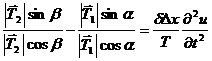
Examples of some important PDEs:

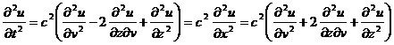
(1) One-dimensional wave equation

(2) One-dimensional heat equation

(3) Two-dimensional Laplace equation

(4) Two-dimensional Poisson equation

Note that for PDEs one typically uses some other function letter such as u instead of y, which now quite often shows up as one of the variables involved in the multivariable function.

In general we can use the same terminology to describe PDEs as in the case of ODEs. For starters, we will call any equation involving one or more partial derivatives of a multivariable function a partial differential equation. The order of such an equation is the highest order partial derivative that shows up in the equation. In addition, the equation is called linear if it is of the first degree in the unknown function u, and its partial derivatives, u_x, u_xx, u_y, etc. (this means that the highest power of the function, u, and its derivatives is just equal to one in each term in the equation, and that only one of them appears in each term). If each term in the equation involves either u, or one of its partial derivatives, then the function is classified as homogeneous.

Take a look at the list of PDEs above. Try to classify each one using the terminology given above. Note that the f(x,y) function in the Poisson equation is just a function of the variables x and y, it has nothing to do with u(x,y).

Answers: all of these PDEs are second order, and are linear. All are also homogeneous except for the fourth one, the Poisson equation, as the f(x,y) term on the right hand side doesn’t involve u or any of its derivatives.

The reason for defining the classifications linear and homogeneous for PDEs is to bring up the principle of superposition. This excellent principle (which also shows up in the study of linear homogeneous ODEs) is useful exactly whenever one considers solutions to linear homogeneous PDEs. The idea is that if one has two functions, and that satisfy a linear homogeneous differential equation, then since taking the derivative of a sum of functions is the same as taking the sum of their derivatives, then as long as the highest powers of derivatives involved in the equation are one (i.e., that it’s linear), and that each term has a derivative in it (i.e. that it’s homogeneous), then it’s a straightforward exercise to see that the sum of and will also be a solution to the differential equation. In fact, so will any linear combination, , where a and b are constants.

For instance, the two functions and are both solutions for the first-order linear homogeneous PDE:

(5)

It’s a simple exercise to check that and are also solutions to the same PDE (as will be any linear combination of and )

This principle is extremely important, as it enables us to build up particular solutions out of infinite families of solutions through the use of Fourier series. This trick is examined in great detail at the end of math 21b, and although we will mention it during the classes on PDEs, we won’t have time in 21a to go into any specifics about the use of Fourier series in this way (so come back for more in Math 21b!)

Solving PDEs

Solving PDEs is considerably more difficult in general than solving ODEs, as the level of complexity involved can be great. For instance the following seemingly completely unrelated functions are all solutions to the two-dimensional Laplace equation:

(1) , and

You should check to see that these are all in fact solutions to the Laplace equation by doing the same thing you would do for an ODE solution, namely, calculate and , substitute them into the PDE equation and see if the two sides of the equation are identical.

Now, there are certain types of PDEs for which finding the solutions is not too hard. For instance, consider the first-order PDE

(2)

where u is assumed to be a two-variable function depending on x and y. How could you solve this PDE? Think about it, is there any reason that we couldn’t just undo the partial derivative of u with respect to x by integrating with respect to x? No, so try it out! This is quite similar to the idea of finding a potential function when one knows the partial derivatives of the function with respect to each of its independent variables. Here, however, we are given information just about one of the partial derivatives, so when we find a solution, there will be an unknown factor that’s not necessarily just an arbitrary constant, but in fact is a completely arbitrary function depending just on y.

To solve (2), then, integrate both sides of the equation with respect to x, as mentioned. Thus

(3)

so that . What is F? Note that it could be any function such that when one takes its partial derivative with respect to x, the result is 0. This means that in the case of PDEs, the arbitrary constants that we ran into during the course of solving ODEs are now taking the form of whole functions. Here F, is in fact any function, F(y),of y alone. To check that this is indeed a solution to the original PDE, it is easy enough to take the partial derivative of this function and see that it indeed satisfies the PDE in (2).

Now consider a second-order PDE such as

(4)

where u is again a two-variable function depending on x and y. We can solve this PDE by integrating first with respect to x, to get to an intermediate PDE,

(5)

where F(y) is a function of y alone. Now, integrating both sides with respect to y yields

(6)

where now G(x) is a function of x alone (Note that we could have integrated with respect to y first, then x and we would have ended up with the same result). Thus, whereas in the ODE world, general solutions typically end up with as many arbitrary constants as the order of the original ODE, here in the PDE world, one typically ends up with as many arbitrary functions in the general solutions.

To end up with a specific solution, then, we will need to be given extra conditions that indicate what these arbitrary functions are. Thus the initial conditions for PDEs will typically involve knowing whole functions, not just constant values. We will also see that the initial conditions that appeared in specific ODE situations have slightly more involved analogs in the PDE world, namely there are often so-called boundary conditions as well as initial conditions to take into consideration.

Examples of PDEs – the Wave Equation

For the rest of this introduction to PDEs we will explore PDEs representing some of the basic types of linear second order PDEs: heat conduction and wave propagation. These represent two entirely different physical processes: the process of diffusion, and the process of oscillation, respectively. The field of PDEs is extremely large, and there is still a considerable amount of undiscovered territory in it, but these two basic types of PDEs represent the ones that are in some sense, the best understood and most developed of all of the PDEs. Although there is no one way to solve all PDEs explicitly, the main technique that we will use to solve these various PDEs represents one of the most important techniques used in the field of PDEs, namely separation of variables (which we saw in a different form while studying ODEs). The essential manner of using separation of variables is to try to break up a differential equation involving several partial derivatives into a series of simpler, ordinary differential equations. Think of this as being analogous to the way we calculated double and triple integrals by breaking them up as iterated integrals involving integration of a single variable at a time.

We start with the wave equation. This PDE governs a number of similarly related phenomena, all involving oscillations. Situations described by the wave equation include acoustic waves, such as vibrating guitar or violin strings, the vibrations of drums, waves in fluids, as well as waves generated by electromagnetic fields, or any other physical situations involving oscillations, such as vibrating power lines, or even suspension bridges in certain circumstances. In short, this one type of PDE covers a lot of ground.

We begin by looking at the simplest example of a wave PDE, the one-dimensional wave equation. To get at this PDE, we show how it arises as we try to model a simple vibrating string, one that is held in place between two secure ends. For instance, consider plucking a guitar string and watching (and listening) as it vibrates. As is typically the case with modeling, reality is quite a bit more complex than we can deal with all at once, and so we need to make some simplifying assumptions in order to get started.

First off, assume that the string is stretched so tightly that the only real force we need to consider is that due to the string’s tension. This helps us out as we only have to deal with one force, i.e. we can safely ignore the effects of gravity if the tension force is orders of magnitude greater than that of gravity. Next we assume that the string is as uniform, or homogeneous, as possible, and that it is perfectly elastic. This makes it possible to predict the motion of the string more readily since we don’t need to keep track of kinks that might occur if the string wasn’t uniform. Finally, we’ll assume that the vibrations are pretty minimal in relation to the overall length of the string, i.e. in terms of displacement, the amount that the string bounces up and down is pretty small. The reason this will help us out is that we can concentrate on the simple up and down motion of the string, and not worry about any possible side to side motion that might occur.

Now consider a string of a certain length, l, that’s held in place at both ends. First off, what exactly are we trying to do in “modeling the string’s vibrations”? What kind of function do we want to solve for to keep track of the motion of string? What will it be a function of? Clearly if the string is vibrating, then its motion changes over time, so time is one variable we will want to keep track of. To keep track of the actual motion of the string we will need to have a function that tells us the shape of the string at any particular time. One way we can do this is by looking for a function that tells us the vertical displacement (positive up, negative down) that exists at any point along the string – how far away any particular point on the string is from the undisturbed resting position of the string, which is just a straight line. Thus, we would like to find a function of two variables. The variable x can measure distance along the string, measured away from one chosen end of the string (i.e. x = 0 is one of the tied down endpoints of the string), and t stands for time. The function then gives the vertical displacement of the string at any point, x, along the string, at any particular time t.

As we have seen time and time again in calculus, a good way to start when we would like to study a surface or a curve or arc is to break it up into a series of very small pieces. At the end of our study of one little segment of the vibrating string, we will think about what happens as the length of the little segment goes to zero, similar to the type of limiting process we’ve seen as we progress from Riemann Sums to integrals.

Suppose we were to examine a very small length of the vibrating string as shown below:

Now what? How can we figure out what is happening to the vibrating string? Our best hope is to follow the standard path of modeling physical situations by studying all of the forces involved and then turning to Newton’s classic equation . It’s not a surprise that this will help us, as we have already pointed out that this equation is itself a differential equation (acceleration being the second derivative of position with respect to time). Ultimately, all we will be doing is substituting in the particulars of our situation into this basic differential equation.

Because of our first assumption, there is only one force to keep track of in our situation, that of the string tension. Because of our second assumption, that the string is perfectly elastic with no kinks, we can assume that the force due to the tension of the string is tangential to the ends of the small string segment, and so we need to keep track of the string tension forces and at each end of the string segment. Assuming that the string is only vibrating up and down means that the horizontal components of the tension forces on each end of the small segment must perfectly balance each other out. Thus

(1)

where T is a string tension constant associated with the particular set-up (depending, for instance, on how tightly strung the guitar string is). Then to keep track of all of the forces involved means just summing up the vertical components of and . This is equal to

(2)

where we keep track of the fact that the forces are in opposite direction in our diagram with the appropriate use of the minus sign. That’s it for “Force,” now on to “Mass” and “Acceleration.” The mass of the string is simple, just , where is the mass per unit length of the string, and is (approximately) the length of the little segment. Acceleration is the second derivative of position with respect to time. Considering that the position of the string segment at a particular time is just , the function we’re trying to find, then the acceleration for the little segment is (computed at some point between a and a +). Putting all of this together, we find that:

(3)

Now what? It appears that we’ve got nowhere to go with this – this looks pretty unwieldy as it stands. However, be sneaky… try dividing both sides by the various respective equal parts written down in equation (1):

(4)

or more simply:

(5)

Now, finally, note that is equal to the slope at the left-hand end of the string segment, which is just evaluated at a, i.e. and similarly equals , so (5) becomes…

(6)

or better yet, dividing both sides by …

(7)

Now we’re ready for the final push. Let’s go back to the original idea – start by breaking up the vibrating string into little segments, examine each such segment using Newton’s equation, and finally figure out what happens as we let the length of the little string segment dwindle to zero, i.e. examine the result as goes to 0. Do you see any limit definitions of derivatives kicking around in equation (7)? As goes to 0, the left-hand side of the equation is in fact just equal to , so the whole thing boils down to:

(8)

which is often written as

(9)

by bringing in a new constant (typically written with , to show that it’s a positive constant).

This equation, which governs the motion of the vibrating string over time, is called the one-dimensional wave equation. It is clearly a second order PDE, and it’s linear and homogeneous.

Solution of the Wave Equation by Separation of Variables

There are several approaches to solving the wave equation. The first one we will work with, using a technique called separation of variables, again, demonstrates one of the most widely used solution techniques for PDEs. The idea behind it is to split up the original PDE into a series of simpler ODEs, each of which we should be able to solve readily using tricks already learned. The second technique, which we will see in the next section, uses a transformation trick that also reduces the complexity of the original PDE, but in a very different manner. This second solution is due to Jean Le Rond D’Alembert (an 18^th century French mathematician), and is called D’Alembert’s solution, as a result.

First, note that for a specific wave equation situation, in addition to the actual PDE, we will also have boundary conditions arising from the fact that the endpoints of the string are attached solidly, at the left end of the string, when x = 0 and at the other end of the string, which we suppose has overall length l. Let’s start the process of solving the PDE by first figuring out what these boundary conditions imply for the solution function, .

Answer: for all values of t, the time variable, it must be the case that the vertical displacement at the endpoints is 0, since they don’t move up and down at all, so that

(1) and for all values of t

are the boundary conditions for our wave equation. These will be key when we later on need to sort through possible solution functions for functions that satisfy our particular vibrating string set-up.

You might also note that we probably need to specify what the shape of the string is right when time t = 0, and you’re right - to come up with a particular solution function, we would need to know . In fact we would also need to know the initial velocity of the string, which is just . These two requirements are called the initial conditions for the wave equation, and are also necessary to specify a particular vibrating string solution. For instance, as the simplest example of initial conditions, if no one is plucking the string, and it’s perfectly flat to start with, then the initial conditions would just be (a perfectly flat string) with initial velocity, . Here, then, the solution function is pretty unenlightening – it’s just , i.e. no movement of the string through time.

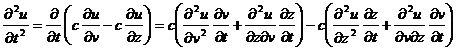
To start the separation of variables technique we make the key assumption that whatever the solution function is, that it can be written as the product of two independent functions, each one of which depends on just one of the two variables, x or t. Thus, imagine that the solution function, can be written as

(2)

where F, and G, are single variable functions of x and t respectively. Differentiating this equation for twice with respect to each variable yields

(3) and

Thus when we substitute these two equations back into the original wave equation, which is

(4)

then we get

(5)

Here’s where our separation of variables assumption pays off, because now if we separate the equation above so that the terms involving F and its second derivative are on one side, and likewise the terms involving G and its derivative are on the other, then we get

(6)

Now we have an equality where the left-hand side just depends on the variable t, and the right-hand side just depends on x. Here comes the critical observation - how can two functions, one just depending on t, and one just on x, be equal for all possible values of t and x? The answer is that they must each be constant, for otherwise the equality could not possibly hold for all possible combinations of t and x. Aha! Thus we have

(7)

where k is a constant. First let’s examine the possible cases for k.

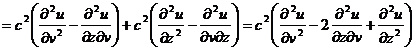
Case One: k = 0

Suppose k equals 0. Then the equations in (7) can be rewritten as

(8) and

yielding with very little effort two solution functions for F and G:

(9) and

where a,b, p and r, are constants (note how easy it is to solve such simple ODEs versus trying to deal with two variables at once, hence the power of the separation of variables approach).

Putting these back together to form , then the next thing we need to do is to note what the boundary conditions from equation (1) force upon us, namely that

(10) and for all values of t

Unless (which would then mean that , giving us the very dull solution equivalent to a flat, unplucked string) then this implies that

(11) .

But how can a linear function have two roots? Only by being identically equal to 0, thus it must be the case that . Sigh, then we still get that , and we end up with the dull solution again, the only possible solution if we start with k = 0.

So, let’s see what happens if…

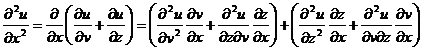
Case Two: k > 0

So now if k is positive, then from equation (7) we again start with

(12)

and

(13)

Try to solve these two ordinary differential equations. You are looking for functions whose second derivatives give back the original function, multiplied by a positive constant. Possible candidate solutions to consider include the exponential and sine and cosine functions. Of course, the sine and cosine functions don’t work here, as their second derivatives are negative the original function, so we are left with the exponential functions.

Let’s take a look at (13) more closely first, as we already know that the boundary conditions imply conditions specifically for , i.e. the conditions in (11). Solutions for include anything of the form

(14)

where and A is a constant. Since could be positive or negative, and since solutions to (13) can be added together to form more solutions (note (13) is an example of a second order linear homogeneous ODE, so that the superposition principle holds), then the general solution for (13) is

(14)

where now A and B are constants and . Knowing that , then unfortunately the only possible values of A and B that work are , i.e. that . Thus, once again we end up with , i.e. the dull solution once more. Now we place all of our hope on the third and final possibility for k, namely…

Case Three: k < 0

So now we go back to equations (12) and (13) again, but now working with k as a negative constant. So, again we have

(12)

and

(13)

Exponential functions won’t satisfy these two ODEs, but now the sine and cosine functions will. The general solution function for (13) is now

(15)

where again A and B are constants and now we have . Again, we consider the boundary conditions that specified that . Substituting in 0 for x in (15) leads to

(16)

so that . Next, consider . We can assume that B isn’t equal to 0, otherwise which would mean that , again, the trivial unplucked string solution. With , then it must be the case that in order to have . The only way that this can happen is for to be a multiple of . This means that

(17) or (where n is an integer)

This means that there is an infinite set of solutions to consider (letting the constant B be equal to 1 for now), one for each possible integer n.

(18)

Well, we would be done at this point, except that the solution function and we’ve neglected to figure out what the other function, , equals. So, we return to the ODE in (12):

(12)

where, again, we are working with k, a negative number. From the solution for we have determined that the only possible values that end up leading to non-trivial solutions are with

for n some integer. Again, we get an infinite set of solutions for (12) that can be written in the form

(19)

where C and D are constants and , where n is the same integer that showed up in the solution for in (18) (we’re labeling with a subscript “n” to identify which value of n is used).

Now we really are done, for all we have to do is to drop our solutions for andinto , and the result is

(20)

where the integer n that was used is identified by the subscript in and , and C and D are arbitrary constants.

At this point you should be in the habit of immediately checking solutions to differential equations. Is (20) really a solution for the original wave equation

and does it actually satisfy the boundary conditions and for all values of t? Check this now – really, don’t read any more until you’re completely sure that this general solution works!

Okay, now what does it mean?

The solution given in the last section really does satisfy the one-dimensional wave equation. To think about what the solutions look like, you could graph a particular solution function for varying values of time, t, and then examine how the string vibrates over time for solution functions with different values of n and constants C and D. However, as the functions involved are fairly simple, it’s possible to make sense of the solution functions with just a little more effort.

For instance, over time, we can see that the part of the function is periodic with period equal to . This means that it has a frequency equal to cycles per unit time. In music one cycle per second is referred to as one hertz. Middle C on a piano is typically 256 hertz (i.e. when someone presses the middle C key, a piano string is struck that vibrates predominantly at 256 cycles per second), and the A above middle C is 440 hertz. The solution function when n is chosen to equal 1 is called the fundamental mode (for a particular length string under a specific tension). The other normal modes are represented by different values of n. For instance one gets the 2^nd and 3^rd normal modes when n is selected to equal 2 and 3, respectively. The fundamental mode, when n equals 1 represents the simplest possible oscillation pattern of the string, when the whole string swings back and forth in one wide swing. In this fundamental mode the widest vibration displacement occurs in the center of the string (see the figures below).

Thus suppose a string of length l, and string mass per unit length , is tightened so that the values of T, the string tension, along the other constants make the value of equal to 440. Then if the string is made to vibrate by striking or plucking it, then its fundamental (lowest) tone would be the A above middle C.

Now think about how different values of n affect the other part of , namely . Since function vanishes whenever x equals a multiple of , then selecting different values of n higher than 1 has the effect of identifying which parts of the vibrating string do not move. This has the affect musically of producing overtones, which are musically pleasing higher tones relative to the fundamental mode tone. For instance picking n = 2 produces a vibrating string that appears to have two separate vibrating sections, with the middle of the string standing still. This mode produces a tone exactly an octave above the fundamental mode. Choosing n = 3 produces the 3^rd normal mode that sounds like an octave and a fifth above the original fundamental mode tone, then 4^th normal mode sounds an octave plus a fifth plus a major third, above the fundamental tone, and so on.

It is this series of fundamental mode tones that gives the basis for much of the tonal scale used in Western music, which is based on the premise that the lower the fundamental mode differences, down to octaves and fifths, the more pleasing the relative sounds. Think about that the next time you listen to some Dave Matthews!

Finally note that in real life, any time a guitar or violin string is caused to vibrate, the result is typically a combination of normal modes, so that the vibrating string produces sounds from many different overtones. The particular combination resulting from a particular set-up, the type of string used, the way the string is plucked or bowed, produces the characteristic tonal quality associated with that instrument. The way in which these different modes are combined makes it possible to produce solutions to the wave equation with different initial shapes and initial velocities of the string. This process of combination involves Fourier Series which will be covered at the end of Math 21b (come back to see it in action!)

Finally, finally, note that the solutions to the wave equations also show up when one considers acoustic waves associated with columns of air vibrating inside pipes, such as in organ pipes, trombones, saxophones or any other wind instruments (including, although you might not have thought of it in this way, your own voice, which basically consists of a vibrating wind-pipe, i.e. your throat!). Thus the same considerations in terms of fundamental tones, overtones and the characteristic tonal quality of an instrument resulting from solutions to the wave equation also occur for any of these instruments as well. So, the wave equation gets around quite a bit musically!

D’Alembert’s Solution of the Wave Equation

As was mentioned previously, there is another way to solve the wave equation, found by Jean Le Rond D’Alembert in the 18^th century. In the last section on the solution to the wave equation using the separation of variables technique, you probably noticed that although we made use of the boundary conditions in finding the solutions to the PDE, we glossed over the issue of the initial conditions, until the very end when we claimed that one could make use of something called Fourier Series to build up combinations of solutions. If you recall, being given specific initial conditions meant being given both the shape of the string at time t = 0, i.e. the function , as well as the initial velocity, (note that these two initial condition functions are functions of x alone, as t is set equal to 0). In the separation of variables solution, we ended up with an infinite set, or family, of solutions, that we said could be combined in such a way as to satisfy any reasonable initial conditions.

In using D’Alembert’s approach to solving the same wave equation, we don’t need to use Fourier series to build up the solution from the initial conditions. Instead, we are able to explicitly construct solutions to the wave equation for any (reasonable) given initial condition functions and .

The technique involves changing the original PDE into one that can be solved by a series of two simple single variable integrations by using a special transformation of variables. Suppose that instead of thinking of the original PDE

(1)

in terms of the variables x, and t, we rewrite it to reflect two new variables

(2) and

This then means that u, originally a function of x, and t, now becomes a function of v and z, instead. How does this work? Note that we can solve for x and t in (2), so that

(3) and

Now using the chain rule for multivariable functions, you know that

(4)

since and , and that similarly

(5)

since and . Working up to second derivatives, another, more involved application of the chain rule yields that

(6)

Another almost identical computation using the chain rule results in the fact that

(7)

Now we revisit the original wave equation

(8)

and substitute in what we have calculated for and in terms of , and . Doing this gives the following equation, ripe with cancellations:

(9)

Dividing by c² and canceling the terms involving and reduces this series of equations to

(10)

which means that

(11)

So what, you might well ask, after all, we still have a second order PDE, and there are still several variables involved. But wait, think about what (11) implies. Picture (11) as it gives you information about the partial derivative of a partial derivative:

(12)

In this form, this implies that considered as a function of z and v is a constant in terms of the variable z, so that can only depend on v, i.e.

(13)

Now, integrating this equation with respect to v yields that

(14)

This, as an indefinite integral, results in a constant of integration, which in this case is just constant from the standpoint of the variable v. Thus, it can be any arbitrary function of z alone, so that actually

(15)

where is a function of v alone, and is a function of z alone, as the notation indicates.

Substituting back the original change of variable equations for v and z in (2) yields that

(16)

where P and N are arbitrary single variable functions. This is called D’Alembert’s solution to the wave equation. Except for the somewhat annoying but easy enough chain rule computations, this was a pretty straightforward solution technique. The reason it worked so well in this case was the fact that the change of variables used in (2) were carefully selected so as to turn the original PDE into one in which the variables basically had no interaction, so that the original second order PDE could be solved by a series of two single variable integrations, which was easy to do.

Check out that D’Alembert’s solution really works. According to this solution, you can pick any functions for P and N such as and . Then

(17)

Now check that

(18)

and that

(19)

so that indeed

(20)

and so this is in fact a solution of the original wave equation.

This same transformation trick can be used to solve a fairly wide range of PDEs. For instance one can solve the equation

(21)

by using the transformation of variables

(22) and

(Try it out! You should get that with arbitrary functions P and N )

Note that in our solution (16) to the wave equation, nothing has been specified about the initial and boundary conditions yet, and we said we would take care of this time around. So now we take a look at what these conditions imply for our choices for the two functions P and N.

If we were given an initial function along with initial velocity function then we can match up these conditions with our solution by simply substituting in into (16) and follow along. We start first with a simplified set-up, where we assume that we are given the initial displacement function , and that the initial velocity function is equal to 0 (i.e. as if someone stretched the string and simply released it without imparting any extra velocity over the string tension alone).

Now the first initial condition implies that

(23)

We next figure out what choosing the second initial condition implies. By working with an initial condition that , we see that by using the chain rule again on the functions P and N

(24)

(remember that P and N are just single variable functions, so the derivative indicated is just a simple single variable derivative with respect to their input). Thus in the case where , then

(25)

Dividing out the constant factor c and substituting in

(26)

and so for some constant k. Combining this with the fact that , means that , so that and likewise . Combining these leads to the solution

(27)

To make sure that the boundary conditions are met, we need

(28) and for all values of t

The first boundary condition implies that

(29)

(30)

so that to meet this condition, then the initial condition function f must be selected to be an odd function. The second boundary condition that implies

(31)

so that . Next, since we’ve seen that f has to be an odd function, then . Putting this all together this means that

(32) for all values of t

which means that f must have period 2l, since the inputs vary by that amount. Remember that this just means the function repeats itself every time 2l is added to the input, the same way that the sine and cosine functions have period 2.

What happens if the initial velocity isn’t equal to 0? Thus suppose . Tracing through the same types of arguments as the above leads to the solution function

(33)

In the next installment of this introduction to PDEs we will turn to the Heat Equation.

Introduction to the Heat Equation

For this next PDE, we create a mathematical model of how heat spreads, or diffuses through an object, such as a metal rod, or a body of water. To do this we take advantage of our knowledge of vector calculus and the divergence theorem to set up a PDE that models such a situation. Knowledge of this particular PDE can be used to model situations involving many sorts of diffusion processes, not just heat. For instance the PDE that we will derive can be used to model the spread of a drug in an organism, of the diffusion of pollutants in a water supply.

The key to this approach will be the observation that heat tends to flow in the direction of decreasing temperature. The bigger the difference in temperature, the faster the heat flow, or heat loss (remember Newton's heating and cooling differential equation). Thus if you leave a hot drink outside on a freezing cold day, then after ten minutes the drink will be a lot colder than if you'd kept the drink inside in a warm room - this seems pretty obvious!

If the function gives the temperature at time t at any point (x, y, z) in an object, then in mathematical terms the direction of fastest decreasing temperature away from a specific point (x, y, z), is just the gradient of u (calculated at the point (x, y, z) and a particular time t). Note that here we are considering the gradient of u as just being with respect to the spatial coordinates x, y and z, so that we write

(1)

Thus the rate at which heat flows away (or toward) the point is proportional to this gradient, so that if F is the vector field that gives the velocity of the heat flow, then

(2)

(negative as the flow is in the direction of fastest decreasing temperature).

The constant, k, is called the thermal conductivity of the object, and it determines the rate at which heat is passed through the material that the object is made of. Some metals, for instance, conduct heat quite rapidly, and so have high values for k, while other materials act more like insulators, with a much lower value of k as a result.

Now suppose we know the temperature function, , for an object, but just at an initial time, when t = 0, i.e. we just know . Suppose we also know the thermal conductivity of the material. What we would like to do is to figure out how the temperature of the object, , changes over time. The goal is to use the observation about the rate of heat flow to set up a PDE involving the function (i.e. the Heat Equation), and then solve the PDE to find .

Deriving the Heat Equation using the Divergence Theorem

To get to a PDE, we invoke, of all things, the divergence theorem! As this is a multivariable calculus topic that we haven’t even gotten to at this point in the semester, don’t worry! Just save these notes for later on this semester and come back to read through this once you’ve learned about the divergence theorem (so for now you can go ahead and skip to the end of this section).

First notice if E is a region in the body of interest (the metal bar, the pool of water, etc.) then the amount of heat that leaves E per unit time is simply a surface integral. More exactly, it is the flux integral over the surface of E of the heat flow vector field, F. Recall that F is the vector field that gives the velocity of the heat flow - it's the one we wrote down as in the previous section. Thus the amount of heat leaving E per unit time is just

(1)

where S is the surface of E. But wait, we have the highly convenient divergence theorem that tells us that

(2)

Okay, now what is div(grad(u))? Given that

(3)

then div(grad(u)) is just equal to

(4)

Incidentally, this combination of divergence and gradient is used so often that it's given a name, the Laplacian. The notation is usually shortened up to simply . So we could rewrite (2), the heat leaving region E per unit time as

(5)

On the other hand, we can calculate the total amount of heat, H, in the region, E, at a particular time, t, by computing the triple integral over E:

(6)

where is the density of the material and the constant is the specific heat of the material (don't worry about all these extra constants for now - we will lump them all together in one place in the end). How does this relate to the earlier integral? On one hand (5) gives the rate of heat leaving E per unit time. This is just the same as , where H gives the total amount of heat in E. This means we actually have two ways to calculate the same thing, because we can calculate by differentiating equation (6) giving H, i.e.

(7)

Now since both (5) and (7) give the rate of heat leaving E per unit time, then these two equations must equal each other, so…

(8)

For these two integrals to be equal means that their two integrands must equal each other (since this integral holds over any arbitrary region E in the object being studied), so…

(9)

or, if we let , and write out the Laplacian, , then this works out simply as

(10)

This, then, is the PDE that models the diffusion of heat in an object, i.e. the Heat Equation! This particular version (10) is the three-dimensional heat equation.

Solving the Heat Equation in the one-dimensional case

We simplify our heat diffusion modeling by considering the specific case of heat flowing in a long thin bar or wire, where the cross-section is very small, and constant, and insulated in such a way that the heat flow is just along the length of the bar or wire. In this slightly contrived situation, we can model the heat flow by keeping track of the temperature at any point along the bar using just one spatial dimension, measuring the position along the bar.

This means that the function, u, that keeps track of the temperature, just depends on x, the position along the bar, and t, time, and so the heat equation from the previous section becomes the so-called one-dimensional heat equation:

(1)

One of the interesting things to note at this point is how similar this PDE appears to the wave equation PDE. However, the resulting solution functions are remarkably different in nature. Remember that the solutions to the wave equation had to do with oscillations, dealing with vibrating strings and all that. Here the solutions to the heat equation deal with temperature flow, not oscillation, so that means the solution functions will likely look quite different. If you’re familiar with the solution to Newton’s heating and cooling differential equations, then you might expect to see some type of exponential decay function as part of the solution function.

Before we start to solve this equation, let’s mention a few more conditions that we will need to know to nail down a specific solution. If the metal bar that we’re studying has a specific length, l, then we need to know the temperatures at the ends of the bars. These temperatures will give us boundary conditions similar to the ones we worked with for the wave equation. To make life a bit simpler for us as we solve the heat equation, let’s start with the case when the ends of the bar, at and both have temperature equal to 0 for all time (you can picture this situation as a metal bar with the ends stuck against blocks of ice, or some other cooling apparatus keeping the ends exactly at 0 degrees). Thus we will be working with the same boundary conditions as before, namely

(2) and for all values of t

Finally, to pick out a particular solution, we also need to know the initial starting temperature of the entire bar, namely we need to know the function . Interestingly, that’s all we would need for an initial condition this time around (recall that to specify a particular solution in the wave equation we needed to know two initial conditions, and ).

The nice thing now is that since we have already solved a PDE, then we can try following the same basic approach as the one we used to solve the last PDE, namely separation of variables. With any luck, we will end up solving this new PDE. So, remembering back to what we did in that case, let’s start by writing

(3)

where F, and G, are single variable functions. Differentiating this equation for with respect to each variable yields

(4) and

When we substitute these two equations back into the original heat equation

(5)

we get

(6)

If we now separate the two functions F and G by dividing through both sides, then we get

(7)

Just as before, the left-hand side only depends on the variable t, and the right-hand side just depends on x. As a result, to have these two be equal can only mean one thing, that they are both equal to the same constant, k:

(8)

As before, let’s first take a look at the implications for as the boundary conditions will again limit the possible solution functions. From (8) we get that has to satisfy

(9)

Just as before, one can consider the various cases with k being positive, zero, or negative. Just as before, to meet the boundary conditions, it turns out that k must in fact be negative (otherwise ends up being identically equal to 0, and we end up with the trivial solution ). So skipping ahead a bit, let’s assume we have figured out that k must be negative (you should check the other two cases just as before to see that what we’ve just written is true!). To indicate this, we write, as before, that , so that we now need to look for solutions to

(10)

These solutions are just the same as before, namely the general solution is:

(11)

where again A and B are constants and now we have . Next, let’s consider the boundary conditions and . These are equivalent to stating that . Substituting in 0 for x in (11) leads to

(12)

so that . Next, consider . As before, we check that B can’t equal 0, otherwise which would then mean that , the trivial solution, again. With , then it must be the case that in order to have . Again, the only way that this can happen is for to be a multiple of . This means that once again

(13) or (where n is an integer)

and so

(14)

where n is an integer. Next we solve for , using equation (8) again. So, rewriting (8), we see that this time

(15)

where , since we had originally written , and we just determined that during the solution for . The general solution to this first order differential equation is just

(16)

So, now we can put it all together to find out that

(17)

where n is an integer, C is an arbitrary constant, and . As is always the case, given a supposed solution to a differential equation, you should check to see that this indeed is a solution to the original heat equation, and that it satisfies the two boundary conditions we started with.

What does it mean?

The next question is how to get from the general solution to the heat equation

(1)

that we found in the last section, to a specific solution for a particular situation. How can one figure out which values of n and C are needed for a specific problem? The answer lies not in choosing one such solution function, but more typically it requires setting up an infinite series of such solutions. Such an infinite series, because of the principle of superposition, will still be a solution function to the equation, because the original heat equation PDE was linear and homogeneous. Using the superposition principle, and by summing together various solutions with carefully chosen values of C, then it is possible to create a specific solution function that will match any (reasonable) given starting temperature function . The way in which we add together solutions involves Fourier series, again, a topic that is too broad to go into at this point, but one which you will see if you continue on with Math 21b!

In any case, you can see one clear feature in the solution functions, which is the presence of the exponential decay term in the solution involving the time variable. For instance, if the temperature at any point on the bar started hotter than the two ends of the bar (which were kept at a steady 0 degrees throughout, according to our boundary conditions), then the exponential decay term shows that as time passes by, the temperature at that point of the bar will exponentially decay down to 0.

To see a particular example in action, you should take a look at the Mathematica assignment on differential equations. In this lab you can enter in different starting functions for the temperature along a metal bar, and see how they decay as t, the time variable increases (look in the section marked “Heat Equation” for details).

Final comments on PDEs

From what you have seen so far in this short introduction to PDEs, it should be clear that knowledge of PDEs is an important part of the mathematical modeling done in many different scientific fields. What you have seen so far is just a small sampling of the vast world of PDEs. In each of the cases we solved, we worked with just the one-dimensional cases, but with a little effort, it is possible to set up and solve similar PDEs for higher-dimensional situations as well. For instance, the two-dimensional wave equation

(1)

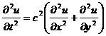
can be used to model waves on the surface of drumheads, or on the surface of liquids, and the three-dimensional heat equation

(2)

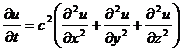
can be used to study temperature diffusion in three-dimensional objects. To solve such equations, one can still use the separation of variables technique that we saw used for the solutions to the one-dimensional cases. However, with more variables involved, one typically has to invoke the technique several times in a row, splitting PDEs involving functions of more than two variables into a sequence of PDEs each involving just one-variable functions. Solutions are then found for each of the one-variable differential equations, and combined to yield solutions to the original PDEs, in much the same way that we saw in the two separation of variables solutions above.

If you would like to learn more about PDEs, and who wouldn’t, then you might want to take a look at one of the classic texts on differential equations, by William Boyce and Richard DiPrima (Elementary Differential Equations and Boundary Value Problems). Another good reference book is Advanced Engineering Mathematics by Erwin Kreyszig (much of this handout was modeled on the approach taken by Kreyszig in his textbook).

Ordinary Differential Equations

Solving Differential Equations

Separation of Variables Technique

Examples

Introduction to Partial Differential Equations

Solving PDEs

Examples of PDEs – the Wave Equation

Solution of the Wave Equation by Separation of Variables

Okay, now what does it mean?

D’Alembert’s Solution of the Wave Equation

Deriving the Heat Equation using the Divergence Theorem

Solving the Heat Equation in the one-dimensional case

What does it mean?

Final comments on PDEs

Suggested Problems