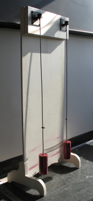
Math21b, Spring 2008, Linear Algebra and Differential Equations,

Pendulum

The pendulum motion is described by the differential equation

 x''(t) = -sin(x)

where x(t) is the angle at time t. For small x, the linearization

 x''(t) = -x

is a good approximation.

Double pendulum

The picture shows the double pendulum borrowed from the Harvard lecture demonstrations. The coupled system of two pendula is

 x''(t) = - x + c (y-x) 
 y''(t) = - y - c (y-x)

The constant c is determined by the spring strength.

Solving the system

This system in vector form is

 v''(t) = A v(t)

with the matrix

A  = | -(1+c)   c    |
     |  c     -(1+c) |

This matrix has the eigenvalues L₁ = -1 with eigenvector v₂ = [1,1]^T and the eigenvalue L₂ = -1-2c with the eigenvector [1,-1]^T.

Write the initial position v(0) = [x(0),y(0)]^T and initial velocity v'(0) = [x'(0),y'(0)]^T as linear combinations of eigenvectors.

v(0)  = a₁ v₁ + a₂ v₂
v'(0) = b₁ v₁ + b₂ v₂

This produces the solution

v(t)  = [ a₁ cos(t) + b₁ sin(t) ] v₁ 
      + [ a₂ cos((1+2c)^1/2 t) + b₂ sin((1+2c)^1/2 t) ] v₂

Eigenmodes

In this system we can "see" the eigenvalues as the squared frequencies of the eigenmodes. One can also see the eigenmodes.
1) Starting with an initial condition where b_i=0 and a₂=0, we have a double pendulum where both pendula swing parallel. The spring strenght does not matter and the penduli move as if they were not connected.
2) Starting with an initial condition where b_i=0 and a₁=0, the pendulum swing against each other. The frequency (1+2c)^1/2 has become slightly larger.


The first eigenmode.	The second eigenmode. It swings a bit faster. The small spring strength makes it swing only slightly faster.	A general initial condition.