Mathematics Math1b
Summer 2003

Introduction to Functions and Calculus II
and Differential equations

"The book of the universe is written in the language of mathematics."

Although the language of mathematics has evolved over time, the statement has as much validity today as it did when it was written. In Mathematics S-1b you will become more vell-versed in the language of modern mathematics and learn about its applications to other disciplines. Math S-1b is a second semester calculus course for students who have previously been introduced to the basic ideas of differential and integral calculus. Over the semester we will study three (related) topics, topics that form a central part of the language of modern science:

• applications and methods of integration,
• infinite series and the representation of functions by infinite polynomials known as power series,
• differential equations.

We begin this course by looking at various applications of the definite integral. The definite integral enables us to tackle many problems, including calculuating the net change in amount given a varying density, determining volume and arclength, and computing physical quantities.

In order to compute integrals we will study some techniques of integration, such as the integration analogues of both the Product Rule and Chain Rule for differentiation. We will briefly look at some alternative transformations of integrals that enable us to tackle them more efficiently. The goal is not to transform you into an integration automaton (we live in the computer age), but to have you acquire familiarity with the techniques and the ability to apply them to some standard situations. More important is the ability to apply the integration as appropriate in problem solving; we will devote time to developing your skill in doing this.

In the second unit of the course we will study infinite sums. You already are aware that a rational number such as can be represented by an infinite sum, ( 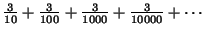, for the case at hand). Actually, irrational numbers such as e and have representations as infinite sums as well. In fact, we will find that many functions, such as f(x) = e^x and can be represented by infinite polynomials known as power series. We will learn to compute, understand, and manipulate these representations. Polynomial approximations based on these power series representations are widely used by engineers, physicists, and many other scientists.

We will end with differential equations, equations modeling rates of change. Differential equations permeate quantitative analysis throughout the sciences (in physics, chemistry, biology, enviromental science, astronomy) and social sciences. In a beautiful and succinct way they provide a wealth of information. By the end of the course you will appreciate the power and usefulness differential equations and you will see how the work we have done with both series and integration comes into play in analyzing their solutions.

Class Meeting Times: Tuesdays and Thursdays 1:00 - 3:30 pm in Science Center 110

Instructor: Robin Gottlieb (gottlieb@math.harvard.edu)

Office: Science Center 429, (617) 495-7882

Office Hours: Tuesdays and Thursdays 3:30 - 4:30 pm

Morning Sessions: Every day: 11:10 am - 12:00 noon in SC 102b.

The daily morning sessions, conducted by Andrew Lobb, are an integral part of the course. All exams except for the final exam will take place in morning sessions.

Text: Stewart's Calculus Concepts and Contexts, 2nd edition. This text is published by Brooks/Cole and is available at the Harvard Coop or via the internet. There will be supplementary material available on the web.

The assumption is that students come into the course having seen most of the material in Chapters 1-4 and 5.1 - 5.5. We'll cover most of Chapters 5-8 plus topics covered in supplementary materials.

Homework: Problems are an integral part of the course; it is virtually impossible to learn the material and to do well in the course without working through the homework problems in a thoughtful manner. Don't just crank through computations and write down answers; think about the problems posed, the strategy you employ, the meaning of the computations you perform, and the answers you get. It is often in this reflection that the greatest learning takes place.

An assignment will be given at each class meeting. Unless otherwise specified, the problem set is due at the following class meeting and will be returned, graded, at the subsequent class. If you miss a class, then you are responsible for obtaining the assignment and handing it in on time. Solutions put together by the course assistant will be available on the course website. When your homework assignments are returned to you, you can consult the solutions for help with any mistakes you might have made. Problem sets must be turned in on time. When computing your final homework grade, your lowest homework score will be dropped.

Note that homework problems will sometimes look a bit different from problems specifically explicitly discussed in class. To do mathematics you need to think about the material, not simply follow recipes. (Following preset recipes is something computers are great at. We want you to be able to do more than this.) Giving you problems different from those done in class is consistent with our goal of teaching you the art of applying ideas of integration and differentiation to different contexts. Feel free to use a calculator or computer to check or investigate problems for homework. However, an answer with the explanation `` because my calculator says so" will not receive credit. Use the calculator as a learning tool, not as a crutch. Calculators will not be allowed on examinations, due in part to equity issues.

You are welcome to collaborate with other students on solving homework problems; in fact, you are encouraged to do so, and we will provided you with contact information for your classmates in order to faciliate that. However, write-ups you hand in must be your own work, you must be comfortable explaining what you have written, and there must be a written acknowledgement of collaboration with the names of you co-workers.

Exams

There will be two exams and one quiz in the morning sessions. Exams must be done without calculators.

Quiz: Tuesday, July 8th 11:10 - 12 noon

Exam 1: Thursday, July 10 from 11-12

Exam 2: Monday, July 28, from 11-12

Grades: The course grades will be based on the two exams (20% each), the final exam (35%), homework (20%), and the technique quiz (5%).

Some notes on emphasis

Integration:

• Everyone should should leave the course having some technical integration skills. Know how and when to use integration by parts and be able to do substitution and partial fraction decomposition. Your knowledge of subtitution must be thorough enough to perform a trigonometric substitution (and realizing that this involves not only transformation of the integrand, but also the `dx' and the endpoints of integration.

• Be able to use reasonability arguments, to estimate size, and to use symmetry arguments; have a geometric interpretation of a integral as well as a computational one.

• Be able to identify problems calling for integration and to be able to set up the appropriate integral without being given a formula to apply. For this reason the process of slicing, approximating a quantity on a slice, summing over all the slices to get a Riemann Sum, and taking the appropriate limit is the real heart of the applications section. The idea is not for students to simply come out with a collection of formulas to apply. (Expect exam questions that cannot be done simply by applying a formula from Thomas' Calculus.)

Series:

When this unit is over I don't want you to think ``Series, isn't that when you have the formulas with all the factorials and you have a bunch of tests you do to determine convergence." Instead, I'd like you to

• think of approximating functions by Taylor polynomials and understand the significance of the `center'
• be happily amazed that many familiar functions have representations as infinite polynomials (power series) whose coefficients are determined by derivatives evaluated at a single point
• have a solid notion of what it means for a series to converge
• be able to apply convergence tests appropriately and have a good grasp of what the alternating series test says, not only in terms of convergence but in terms of error
• understand the idea of radius of convergence of a power series and be comfortable manipulating power series using substitution, integration, and differentiation.

Differential Equations:

The main ideas and skills you should take away from this part of the course include:

• modeling a situation using a differential equation or system of differential equations
• knowing what it means to be a solution to a differential equation
• being able to do qualitative analysis of solutions and being able to interpret solutions (particularly for autonomous differential equations and systems.
• solving separable differential equations, first order linear differential equations and 2nd order homogeneous differential equations with constant coefficients and being able to interpret these solutions.

TENTATIVE DAY-BY-DAY SYLLABUS: Summer, 2003

Topics are indicated by the dates and corresponding sections in the text and supplement are given. `S' indicates reading in Stewart's Calculus and `G' indicates reading in the supplement by the instructor. Italics are used to indicate optional reading.

1.

Tues. June 24:

Areas, density and slicing. Total mass from density; total population from population density.

[ S: 6.1 G: 27.1]

2.

Thurs. June 26:

Volumes, volumes of revolution, arclength, average value. Begin work.

[ S: 6.2, 6.3, 6.4, and parts of 6.5 G: 24.2, 28.1, parts of 28.2 ]

3.

Tues. July 1:

Work: pulling, pushing, and pumping.

Integration techniques: substitution (the Chain Rule in reverse) and integration by parts (the counterpart of the Product Rule).

[ S: 6.5 (on work) 5.5 and 5.6 G: parts of 28.2 plus 25.2, 29.1 ]

4.

Thurs. July 3:

Partial fractions, improper integrals, and a lead into series.

[ S: 5.7, 5.10 G: 29.3, 29.4 ]

5.

Tues. July 8:

Motivation. Sequences and Infinite Series. Geometric sums and geometric series. Nth Term Test for Divergence. Introduction to comparison analysis.

[ S: 8.1, 8.2 ]

Thursday, July 10th Exam 1: Topic: Integration SC 102b

6.

Thurs. July 10:

Taylor polynomials: approximating a function by a polynomial.

Taylor series: representing a function by a power series.

[ S: 8.6 G: 30.1, parts of 30.2, 30.3 ]

7.

Tues. July 15:

Convergence tests:

The Integral test, Comparison Tests, Alternating Series Test, absolute convergence, and the Ratio Test.

[ S: 8.3, 8.4 G: 30.5]

8.

Thurs. July 17:

Re-cap of convergence criteria. Power Series, Taylor and Maclaurin series.

[ S: 8.5, 8.6, 8.7 G: 30.4 ]

9.

Tues. July 22:

More power series and Taylor series.

[ S: 8.8, 8.9 ]

10.

Thurs. July 24:

Modeling with differential equations. Solutions to differential equations.

Slope fields. ,     ,     ,    and . Guess and check solutions.

[ S:7.1, 7.2 G: 31.1, 31.2]

Monday, July 28th Exam 2: Topic: Series

11.

Tues. July 29:

Separation of variables, Mixture problems. Qualitative solutions to autonomous first order linear differential equations.

[ S: 7.3 G: 31.3, 31.4 ]

12.

Thurs. July 31:

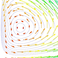
Systems of differential equations.

[ S: 7.6, G: 31.5]

13.

Tues. August 5:

Vibrating springs and second order linear homogeneous differential equations with constant coefficients.

[ G: 31.6]

14.

Thurs. August 7:

Series solutions to differential equations. Additional topics to be determined. (Perhaps solving first order linear differential equations, or Euler's method.)

[ S: 8.10]

Tuesday, August 12: 1:30 - 4:30 pm Final Examination