Maurer Roses
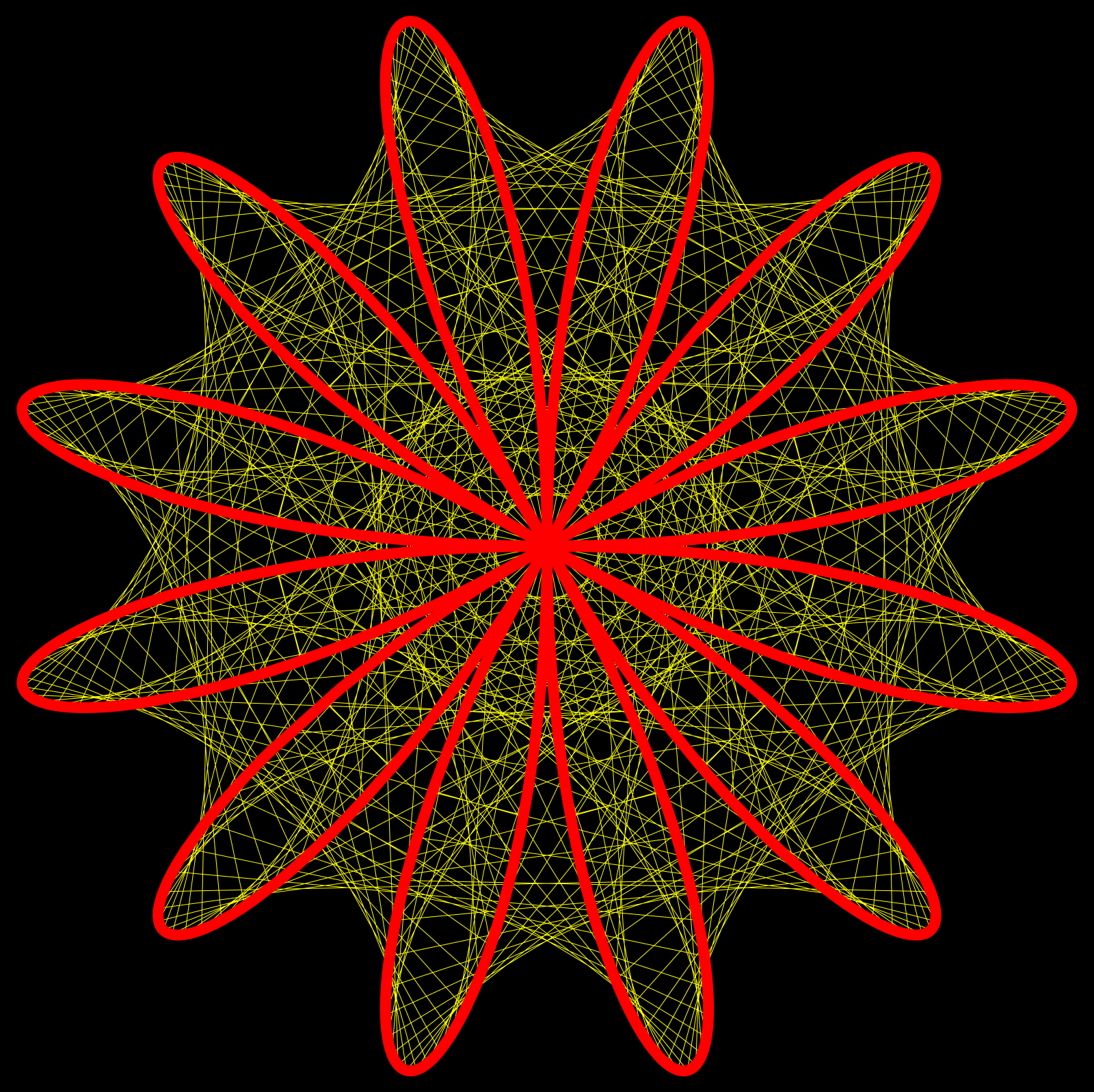
A rose is the polar curve, where the radius at angle t is sin(n t). Its parametrization in two dimensions isr(t) = < sin(nt) cos(t), sin(nt) sin(t) >A Maurer rose is a polygonal curve connecting the points r(k a), where a is an angle. The pictures can be generated quickly with Mathematica. Here is one of the pictures you find on the Wikipedia page:
n=6; d=71; M=500;    r[t_]:=Sin[n*t]{Cos[t],Sin[t]};
S1=ParametricPlot[r[t],{t,0,2Pi},PlotStyle->{Thickness[0.01],Red}];
S2=Graphics[{Blue,Line[Table[r[t*Pi*d/180],{t,0,M}]]}];Show[{S2,S1}]
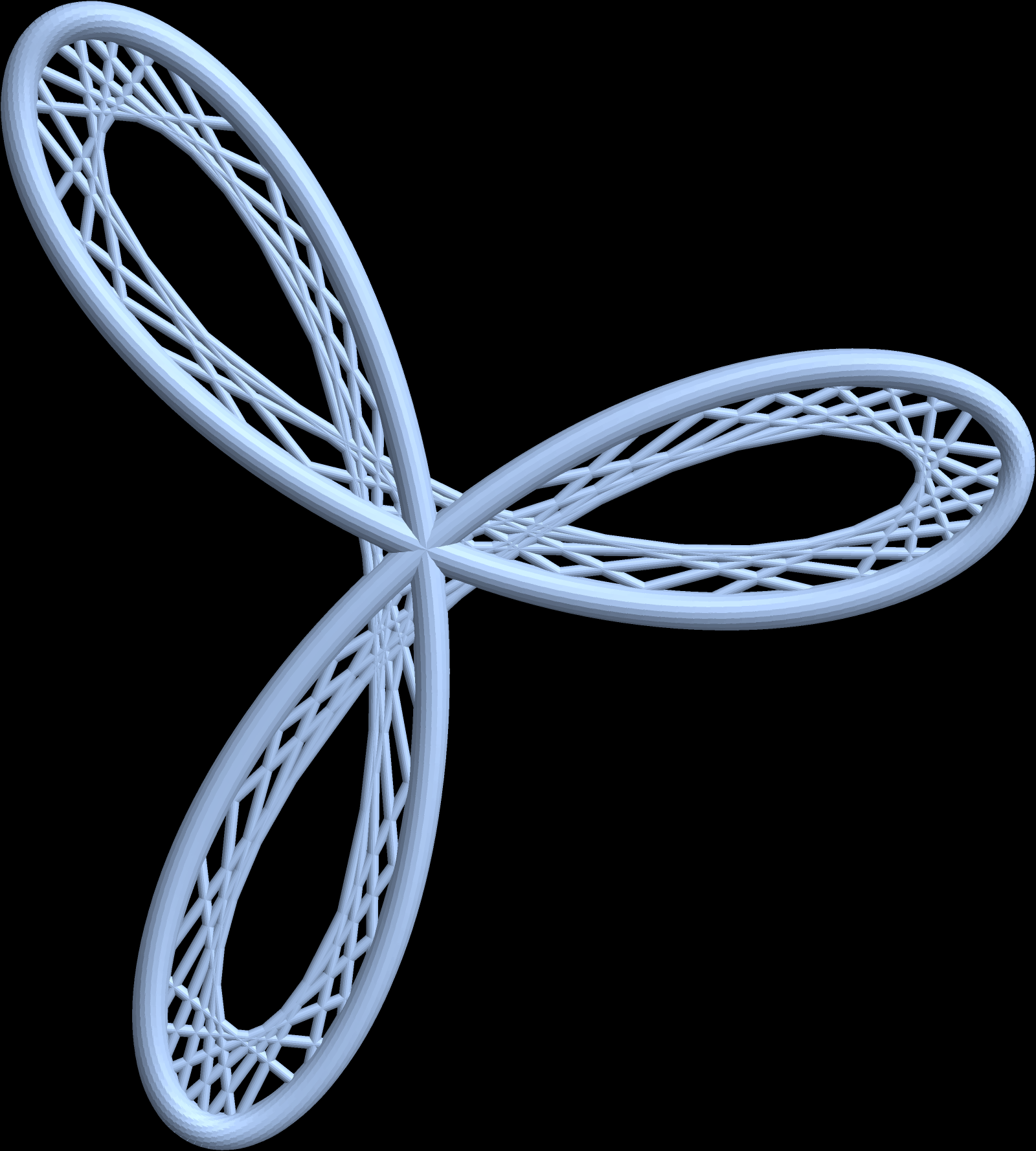
n=2; d=31; M=100; r[t_]:=Sin[n*t]{Cos[t],Sin[t],0}; Show[{
Graphics3D[{Orange,Tube[Table[r[t], {t,0,2*Pi,0.01}],0.03]}],
Graphics3D[{Blue,Tube[Table[r[t*Pi*d/180],{t,0,M}],0.01]}]}]

Assume we want to 3D print a rose, we just can export it as "STL":r[t_]:=Sin[2*t]{Cos[t],Sin[t],0};Graphics3D[ Tube[{Table[r[t],{t,0,2Pi,0.01}],Table[r[t*Pi*31/180],{t,0,99}]},0.01]] pic.twitter.com/uQknxzGuA1
— Harvard 21a Calculus () September 15, 2016
n = 3; d = 21; M = 50; r[t_]:=Sin[n*t] {Cos[t], Sin[t], 0};
S1=Graphics3D[Tube[Table[r[t], {t, 0, 2 Pi, 0.01}], 0.03]];
S2=Graphics3D[Tube[Table[r[t*Pi*d/180], {t, 0, M}], 0.01]];
Export["rose.stl",Show[{S1, S2}],"STL"]
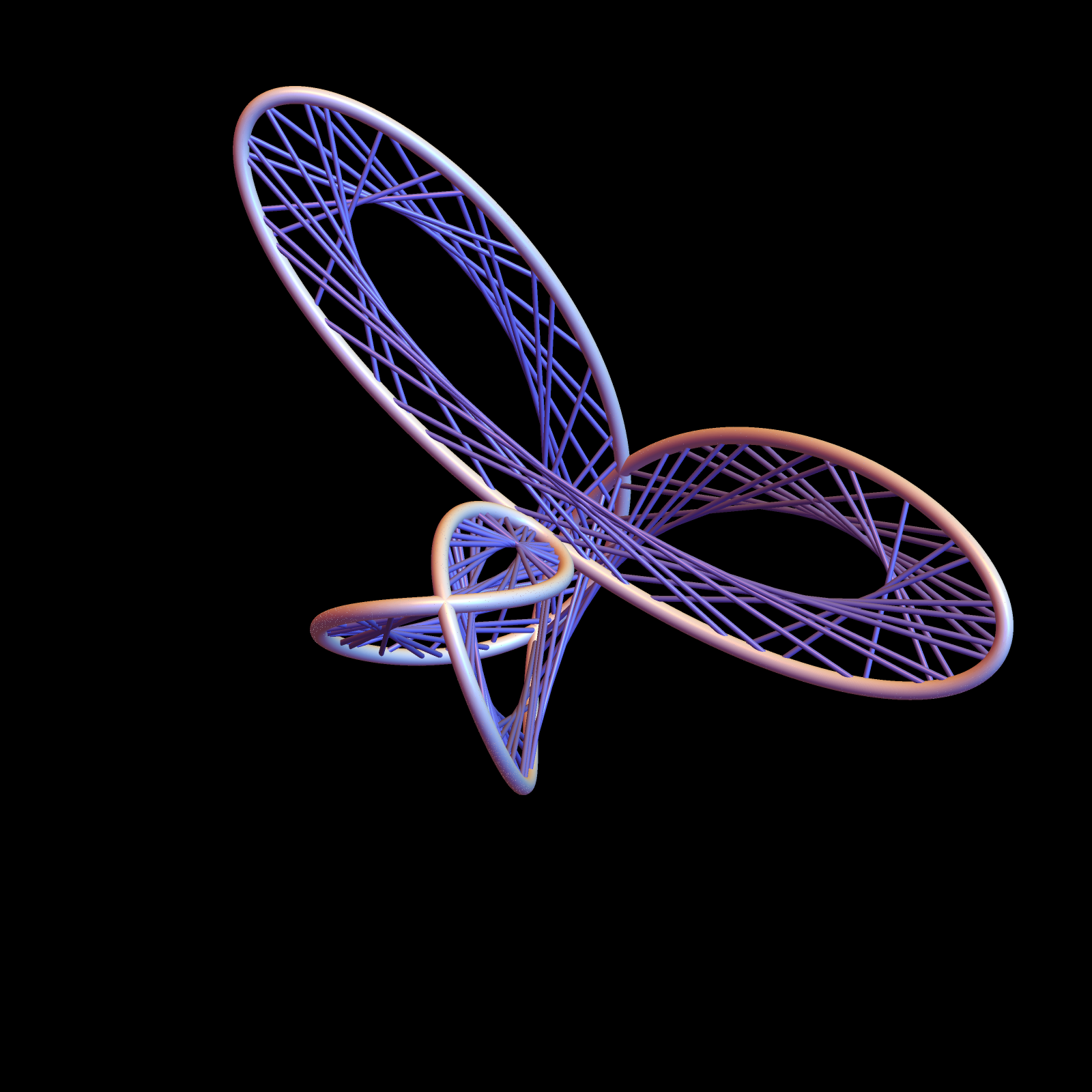
 r1(t) = < sin(n1 t) cos(t), sin(n1 t) sin(t),0 >
 r2(t) = < sin(n2 t) cos(t), 0, sin(n2 t) sin(t)>
 r(t)  = r1(t) + r2(t)
And here is the Mathematica code which produces the sum. And why use 5 lines of code for that if you can do it in 4 lines?
n1=2; n2=3; d=31; M=100; r1[t_]:=Sin[n1*t]{Cos[t],Sin[t],0};
r2[t_]:=Sin[n2*t]{Cos[t],0,Sin[t]}; r[t_]:=r1[t]+r2[t]; Show[{
Graphics3D[{White,Tube[Table[r[t], {t, 0,2Pi,0.001}],0.03]}],
Graphics3D[{Blue, Tube[Table[r[t*Pi*d/180],{t,0,M}],0.01]}]}]