Area of the Mandelbrot set

For background, look at the Monte Carlo Mandelbrot exhibit from Fall 2019 with a bit of Write up on the area of the Mandelbrot set [PDF]. Or the Mandelbrot Zoom from 2018 which you have to see full screen! Here are the results reported by the rare element groups. We see that there is an obvious correlation between the number of iterations and the area. Of course, if one runs the iterations longer, more points are melted away from the set considered in the Mandelbrot set. The Decimal expansion of the area of the Mandelbrot set is called A098403. It is there reported to start with 1.506591. Here are the results reported by the rare elements:

Group              Iter   Runs        Result
---------------------------------------------
Gadolinium         1000   1000000     1.51188
Actinium           10000  10000000    1.50818
Neodynimum         1000   7000000     1.51016
Terbium            5000   900000      1.50875
Yttrium            2000   5000000     1.50843
Ytterbium          1000   10000000    1.50791
Thorium            2000   1000000     1.50803       
Dysposium          1000   2500000     1.51132
Lutetium           500000 1000000     1.50774
Erbium             1000   1000000000  1.51026
Europium           1000   10000000    1.50940
Samarium           4000   10000000    1.50869
Cerium             10000  10000000    1.50756
Praseodymium       1000   2500000     1.51132
Holmium            1000   10000000    1.50999
Lutetium           1000   1000000000  1.51036
Scandium           50000  10000000    1.50673
Lanthanum          5000   10000000    1.50687 
Promethium         1000   10000000    1.50945

Here is some comparison which I ran on three of my machines: (the knill12 job was running July 20 to July 28)

Oliver: knill12    2000   2262600000  1.50834
Oliver: knill12    2000   6742800000  1.50839  (August 11)
Oliver: knill27   12000   37730000    1.50768
Oliver: knill11    1200   395900000   1.50979

It uses code which does the computation in smaller steps and reports out. I save this as a file "mandelbrotarea.m", then run in a terminal "nohup math < mandelbrotarea.m > out &" which will continue running the job and continuously write onto the file out. This can then be distributed onto other machines.

T=0; Do[ m=10000; n=12000;
  M=Compile[{x,y},Module[{z=x+I y,k=0},
   While[Less[Abs[z],2] && Less[k,n],z=N[z^2+x+I y];++k];Floor[k/n]]];
  U=9*Sum[M[-2.0+3 Random[],-1.5+3 Random[]],{m}]/m;
  T=T+U; Print[{t,U,N[T/t]}], {t,1000000}]

Sebastian Ingino wrote some Python code for Google Colab and got the following result:

Samarium(Python)   20000  10000000    1.505724

Here is the project page of Sebastian on Colab.research.google. Update of July 28: Sebastian has increased the speed using Tensorflow and running on Tensorflow-optimized hardware. . This is about 30x faster when using 2000 iterations and 1000000 samples and uses only 3 seconds to run. The Mathematica job, I have been running since more than a week would be done in 10 minutes. Here is the Python code (simplified from Sebastians page) without multi-processing: just save it as file mandelbrotarea.py and run python < mandelbrotarea.py on a terminal. mandelbrotarea.txt [TXT file]

from numpy import random
import math

iterations = 2000
samples = 100000

def M(x,y):
    z = x+y*1j
    k = 0
    while abs(z) < 2 and k < iterations:
      z = z*z+ x+y*1j
      k += 1
    return math.floor(k/iterations)

sum = 0
n = 0
while n < samples:
   n += 1
   sum += M(-2 + 3*random.rand(), -1.5 +3*random.rand())

final = 9*sum/samples
print(final);

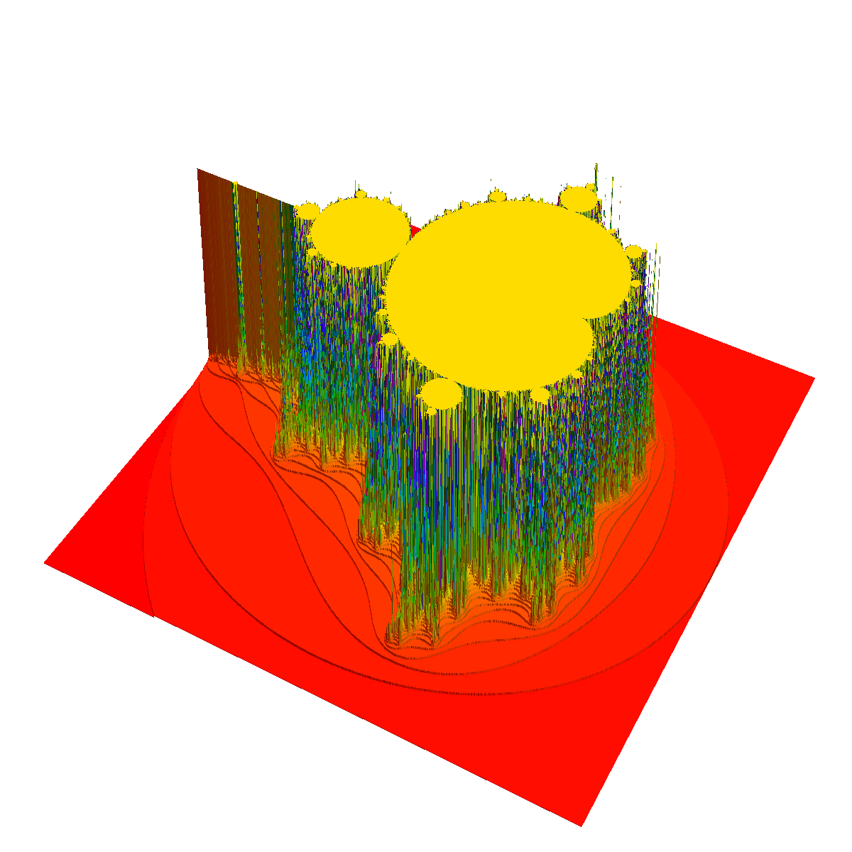
Here is a 3D plot of the Mandelbrot set

M=Compile[{x,y},Module[{z=x+I y,k=0,n=200},
   While[Less[Abs[z],2] && Less[k,n],z=N[z^2+x+I y];++k];k/n]];
Plot3D[M[x,y],{x,-2,1},{y,-1.5,1.5},PlotPoints->300,ColorFunction->Hue]

Math 21a Summer 2020

Multivariable Calculus

Area of the Mandelbrot set